The advection-diffusion-reaction equation

The advection-diffusion-reaction equation (also called the continuity equation in semiconductor physics) in flux form, is given by,

\[u_t = (\mathcal{-F})_x + s(t,x,u)\]

where \(\mathcal{F} = au - du_x\). This expression holds over the whole domain, therefore it must also hold over a subdomain \(\Omega_j=(x_{j-1/2}, x_{j+1/2})\). Integrating over the subdomain, or cell, gives,

\[\int_{x_{j-1/2}}^{x_{j+1/2}} u_t~dx = \int_{x_{j-1/2}}^{x_{j+1/2}} (\mathcal{-F})_x~dx + \int_{x_{j-1/2}}^{x_{j+1/2}} s(x,t,u)~dx\]

If we now use \(w\) and \(\bar{s}\) to represent the cell averages of the solution variable and reaction term then we don’t have to perform any actual integrations. The fundamental quantity we will use in the discretised equations is a cell average,

\[w_j^{\prime} = -\frac{\mathcal{F}_{j+1/2}}{h_j} + \frac{\mathcal{F}_{j-1/2}}{h_{j}} + \bar{s}_j\]

Note

In the above we can perform the integration of the flux term. Integrating the divergence of the flux over the unit cell simply gives use the flux at the cell faces, \(\int_{x_{j-1/2}}^{x_{j+1/2}} (\mathcal{-F})_x~dx = \left[ \mathcal{-F} \right]_{x_{j-1/2}}^{x_{j+1/2}}\). Because we want the cell average we divide by the cell width \(h_j\). In three dimension we would divide by the volume of the cell, hence the name, finite volume method.

For the advection component of the flux we will use a linear interpolation (see Aside: Linear interpolation between cell centre and face values) to determine the contribution at the cell faces, and for the diffusion component with will use a simple cell average,

\[\mathcal{F}_{j+\frac{1}{2}} = a_{j+\frac{1}{2}}\left( \frac{h_{j+1}}{2h_{+}} w_j + \frac{h_j}{2h_{+}} w_{j+1} \right) - d_{j+\frac{1}{2}} \frac{w_{j+1}-w_j}{h_{+}}\]

\[\mathcal{F}_{j-\frac{1}{2}} = a_{j-\frac{1}{2}}\left( \frac{h_{j}}{2h_{-}} w_{j-1} + \frac{h_{j-1}}{2h_{-}} w_{j} \right) - d_{j-\frac{1}{2}} \frac{w_{j}-w_{j-1}}{h_{-}}\]

The meaning of the “h” terms is shown in the figure below,

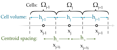
Finite volume cells with important distances and positions labelled.

Substituting the definition of the fluxes into the above equation yields,

(1)\[w_j^{\prime} = \frac{w_{j-1}}{h_j} \left( \frac{a(x_{j-\frac{1}{2}}) h_j}{2h_{-}} + \frac{d(x_{j-\frac{1}{2}})}{h_{-}}\right) + \frac{w_j}{h_j}\left( \frac{a(x_{j-\frac{1}{2}})h_{j-1}}{2h_{-}} - \frac{a(x_{j+\frac{1}{2}})h_{j+1}}{2h_{+}} - \frac{d(x_{j-\frac{1}{2}})}{h_{-}} - \frac{d(x_{j+\frac{1}{2}})}{h_{+}} \right) + \frac{w_{j+1}}{h_j} \left( \frac{-a(x_{j+\frac{1}{2}})h_j}{2h_{+}} + \frac{d(x_{j+\frac{1}{2}})}{h_{+}} \right)\]

This equation is the semi-discrete form because the equation has not been discretised in time.

For convenience we will simply write the r.h.s. of (1) as,

\[w_j^{\prime} = F(w)\]

where it is understood that \(w = (w_{j-1}, w_j, w_{j+1})\) stands for the discretisation stencil.

Adaptive upwinding & exponential fitting

Hundsdorfer (on pg. 266) notes that a adaptive upwinding scheme can be introduced by altering the diffusion coefficient,

\[d(x_{j}) \rightarrow d(x_{j}) + \frac{1}{2}\kappa_{j} h_{j} a(x_{j})\]

\[\kappa=\text{sgn}(a(x_{j})).\]

Here the nature of the discretisation is defined by the sign of the \(a\), when \(a\neq0\) the scheme results in an upwind discretisation. Only if \(a=0\) (corresponding to the diffusion equation limit) does the scheme become based on a central difference (see the red line in the Figure below). A generalisation is possible by choosing a function for \(\kappa\) which automatically adjusts the discretisation method depending on the local value of Peclet’s number, \(\mu=ah/d\). Exponential fitting has shown to be a robust scheme for steady-state approaches. Exponential fitting can be introduced by,

\[\kappa = \frac{e^{\mu}+1}{e^{\mu}-1} - \frac{2}{\mu}\]

An approximation to the above, which does not require the evaluation of exponentials is commonly used,

\[\begin{split}\kappa = \begin{cases} \text{max}(0, 1-2/\mu) & \text{when}~ \mu>0 \\ \text{min}(0, -1-2/\mu) & \text{when}~ \mu<0 \end{cases}\end{split}\]

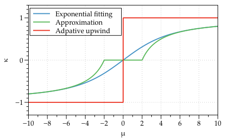
This is a very elegant want to introduce adaptive upwinding or exponential fitting because it can be brought into the discretisation in an ad hoc manner. Note that for all of the adaptive expressions \(\kappa\rightarrow\pm1\) as \(\mu\rightarrow\pm\infty\), and \(\kappa\rightarrow 0\) as \(\mu\rightarrow 0\). This means the discretisation will automatically weight in the favour of the upwind scheme in locations where advection dominates. Conversely, where diffusion dominates the weighting factor shifts in favour of a central difference scheme.

Explicit and implicit forms

In the discussion so far we have been ignoring one important deal: at what time is the r.h.s of the discretised equation evaluated?

Moreover, if we choose the r.h.s to be evaluated at the present time step, \(t_n\) this is known as an explicit method,

\[w_j^{\prime} = F(w^n)\]

Explicit methods are very simple. Starting with initial conditions at time \(t_n\), the above equation can be rearranged to find the solution variable \(w_j^{n+1}\) at the future time step, \(t_{n+1}\).

However the downside of using explicit methods is that they are often numerically unstable unless the time step is exceptionally (sometime unrealistically) small.

Fortunately there is an second alternative, we can choice to write the r.h.s of the equation at the future time step, \(t_{n+1}\), this is known as an implicit method,

\[w_j^{\prime} = F(w^{n+1})\]

Explicit methods are significantly more numerically robust, however they pose a problem, how does one write the equations because the solution variable at the future time step \(w^{n+1}\) is unknown? The answer is that at each time step we must solve a linear system of equation to find \(w^{n+1}\).

Note

For the linear advection-diffusion-reaction equation implicit methods are simply to implement even though the computation cost is increases. One must simply write the equation in the linear form \(A\cdot x = d\) and solve for \(x\) which is the solution variable at the future time step. However if the equations are non-linear then implicit methods pose problem because the equation cannot be written in linear form. In these situations are there are a number of techniques that are used but they all most use a iterative procedure, such as a Newton-Raphson method, to solve the equations.

The following section assumes that the equation is linear.

The \(\theta\)-method

The \(\theta\)-method is an approach which combines implicit and explicit forms into one method. It consists of writing the equation as the average of the implicit and explicit forms. If we let \(F_{w^{n}}\) and \(F_{w^{n+1}}\) stand for the r.h.s of the explicit and implicit forms of the equations then the \(\theta\)-method gives,

\[w_j^{\prime} = \theta F(w_j^{n+1}) + (1-\theta)F(w_j^{n})\]

Setting \(\theta=0\) recovers a fully implicit scheme while \(\theta=1\) gives a fully explicit discretisation. The value of \(\theta\) is not limited to just 0 or 1. It is common to set \(\theta=1/2\), this is called the Crank-Nicolson method. It is particularly popular for diffusion problem because it preserves the stability of the implicit form but also increases the accuracy of the time integration from first to second order (because two points in time are being averaged). For advection diffusion problems the Crank-Nicolson method is also unconditionally stable.

In the above equation,

\[\begin{split}F(w_j^{n}) = r_a w_{j-1}^{n} + r_b w_{j}^{n} + r_c w_{j+1}^{n} \\ F(w_j^{n+1}) = r_a w_{j-1}^{n+1} + r_b w_{j}^{n+1} + r_c w_{j+1}^{n+1}\end{split}\]

and the coefficients are,

\[\begin{split}r_a & = \frac{1}{h_j} \left( \frac{a(x_{j-\frac{1}{2}}) h_j}{2h_{-}} + \frac{d(x_{j-\frac{1}{2}})}{h_{-}}\right) \\ r_b & = \frac{1}{h_j}\left( \frac{a(x_{j-\frac{1}{2}})h_{j-1}}{2h_{-}} - \frac{a(x_{j+\frac{1}{2}})h_{j+1}}{2h_{+}} - \frac{d(x_{j-\frac{1}{2}})}{h_{-}} - \frac{d(x_{j+\frac{1}{2}})}{h_{+}} \right)\\ r_c & = \frac{1}{h_j} \left( \frac{-a(x_{j+\frac{1}{2}})h_j}{2h_{+}} + \frac{d(x_{j+\frac{1}{2}})}{h_{+}} \right)\end{split}\]

We have written the coefficients without dependence on time to simplify the notation, but the coefficients should be calculated at the same time points as their solution variable. However, the coefficients must be linear, they should not depend on the values of the solution variable.

Discretised equation in matrix form

Dropping the spatial subscripts and writing in vector form the equations becomes,

\[\begin{split}\frac{w^{n+1} - w^{n}}{\tau} & = \theta F(w^{n+1}) + (1-\theta)F(w^{n})\end{split}\]

where,

\[\begin{split}F(w^{n+1}) = M^{n+1} w^{n+1} + s^{n+1} \\ F(w^{n}) = M^{n}w^{n} + s^{n}\end{split}\]

with the coefficient matrix,

\[\begin{split}M = \begin{align} \begin{pmatrix} r_b & r_c & & & 0 \\ r_a & r_b & r_c & & \\ & \ddots & \ddots & \ddots& \\ & & r_a & r_b & r_c \\ 0 & & & r_a & r_b \end{pmatrix} \end{align}\end{split}\]

The \(r\)-terms have be previously defined as the coefficients that result from the discretisation method. Note that the subscripts for the \(r\)-terms have been dropped to simplify the notation, but they are functions of space. For example, terms in the first row should be calculated with \(j=1\), in the second with \(j=2\) etc. Solving linear equations is discussed late in section XX.

Aside: Linear interpolation between cell centre and face values

In general, linear interpolation between two points \((x_0, x_1)\) can be used to find the value of a function at \(f(x)\),

\[f(x) = \frac{x - x_1}{x_0 - x_1}f(x_0) + \frac{x - x_0}{x_1 - x_0}f(x_1)\]

In a cell centred grid we know the value of the variable \(w\) at difference points, \(w_j\) and \(w_{j+1}\). We can apply the linear interpolation formulae above to determine value at cell face \(w_{j+1/2}\).

\[w_{j+1/2} = \frac{x_{j+1/2} - x_{j+1}}{x_{j} - x_{j+1}} w_j + \frac{x_{j+1/2} - x_j}{x_{j+1} - x_j} w_{j+1}\]

This can be simplified firstly by using function to represent the distance between cell centres,

\[h_{-} = x_j - x_{j-1} \quad h_{+} = x_{j+1} - x_{j}\]

to give,

\[w_{j+1/2} = \frac{x_{j+1} - x_{j+1/2}}{h_{+}} w_j + \frac{x_{j+1/2} - x_j}{h_{+}} w_{j+1}\]

This expression still contains \(x_{j+1/2}\) which we can simplify further by using an expression for the position of cell centres,

\[x_j = \frac{1}{2} \left( x_{j-\frac{1}{2}} + x_{j+\frac{1}{2}} \right) \quad x_{j+1} = \frac{1}{2} \left( x_{j+\frac{1}{2}} + x_{j+\frac{3}{2}} \right)\]

Note, this expression is still valid of non-uniform grids, it simply says that cell centres are always equidistant from two faces. Rearranging the above expression and substituting in for \(x_{j}\) and \(x_{j+1}\) terms gives,

\[w_{j+1/2} = \frac{\frac{1}{2} \left( x_{j+\frac{1}{2}} + x_{j+\frac{3}{2}} \right) - x_{j+1/2}}{h_{+}} w_j + \frac{x_{j+1/2} - \frac{1}{2} \left( x_{j-\frac{1}{2}} + x_{j+\frac{1}{2}} \right)}{h_{+}} w_{j+1}\]

Finally, by defining the distance between vertices as, \(h_j = x_{j+\frac{1}{2}} - x_{j-\frac{1}{2}}\), we can simplify to the following expression,

\[w_{j+1/2} = \frac{h_{j+1}}{2h_{+}} w_j + \frac{h_j}{2h_{+}} w_{j+1}\]

Similarly the \(w_{j-1/2}\) can be found,

\[w_{j-1/2} = \frac{h_{j}}{2h_{-}} w_{j-1} + \frac{h_{j-1}}{2h_{-}} w_{j}\]