Solving linear equations

Provided the equation is linear, meaning that the coefficients, nor the reaction term depend on the solution variable a time-stepping approach can be used to solve the equation.

Time stepping the advection-diffusion equation

Here we will rearrange the \(\theta\)-method form of the advection-diffusion equation,

\[\begin{split}\frac{w^{n+1} - w^{n}}{\tau} & = \theta F(w^{n+1}) + (1-\theta)F(w^{n})\end{split}\]

into the form of a linear system \(A\cdot x = d\). Firstly lets move all terms involving future time points the l.h.s,

\[w^{n+1} - \theta \tau F(w^{n+1}) = w^{n} + (1-\theta) F(w^{n+1})\]

Replacing the \(F\) terms with the full matrix expressions and factoring yields,

\[\underbrace{(I - \theta\tau M^{n+1})}_{A}\underbrace{w^{n+1}}_{x} = \underbrace{(I + (1-\theta)\tau M^{n})w^{n}}_{d}\]

Time-stepping involves solving this equation iteratively. First the initial conditions \(w^0\) is used to calculate the solution variable at the next point in time \(w^1\), then values of the solution variable are updated such that \(w^1\) is used to calculate \(w^2\), and so on and so forth. This procedure is shown in the Figure below,

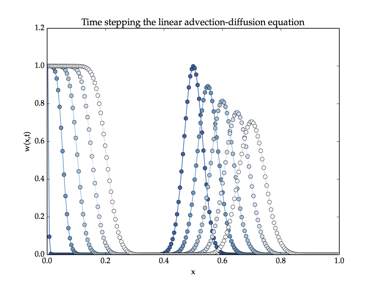
Note

Parameters used for this simulation. \(a=1\), \(d=1\times 10^{-3}\), \(h=5 \times 10^{-3}\), \(\tau=5 \times 10^{-4}\) with exponentially fitted discretisation. The initial and boundary conditions where, \(u(x,t_{0}) =sin(\pi x)^{100}\) with \(u(x_1)=1\) and \(u_x(x_J)=0\). The equation was time stepped for 400 iterations, the plots so the solution at times \(t=0,0.05,0.1,0.15,0.2\).