Solving nonlinear equations

Note

Nonlinear equations are defined as those having coefficients which are functions of the solution variable.

In the previous section we discussed how to solve the linear advection-diffusion-reaction equation with method of time stepping. We used the Crank-Nicolson scheme: the implicit terms provides stability (unrestricted time step) and by also using the explicit term the accuracy of the time integration is improved to second order. However, this approach is only valid for linear equations.

Nonlinear equations (by definition) cannot be written in linear form, as such the time-stepping approach cannot be used. It remains possible to use a fully explicit method, however in practice this is usually not done because the time step is too restrictive or the explicit form is unconditionally unstable.

Here we discuss three approach which can be used to solve nonlinear equations:

1. IMEX (implicit/explicit) time-stepping
2. Newton iteration
3. Method of lines

Fisher’s equation

We will use Fishers’ nonlinear reaction-diffusion equation as an example because it has an analytical solution,

\[u_t = d u_{xx} + \beta u(1 - u)\]

We can directly apply the discretisation scheme already developed, but we must set \(a=0\) and note the nonlinear reaction term \(\beta u(1 - u)\). With semi-open boundary condition \(u(x_0,t)=1\) Fishers’ equation has the analytical form,

\[\begin{split}u(x,t) = \frac{1}{\left(1 + e^{c^{1/2}\left(x - Ut\right)} \right)^2} \\\end{split}\]

where \(U = 5\left(\frac{1}{c}\right)^{1/2}\), and, \(c=\frac{6}{d\beta}\)

IMEX time-stepping

The IMEX scheme treats the linear parts of the equation using implicit (or semi-implicit) scheme and the non-linear parts full explicitly. Therefore for Fishers’ equation this becomes,

\[w^{\prime} = \theta M^{n+1}u^{n+1} + (1-\theta) M^{n}u^{n} + \beta u^n(1-u^n)\]

This can be rearranged into the form \(A\cdot x = d\) and solved by standard time stepping techniques. First we discretised the time derivative \(u^{\prime} = \frac{u^{n+1} - u^{n}}{\tau}\), then we rearrange the equation so that future time points are on the l.h.s. and known time points are on the right,

\[u^{n+1} - \theta \tau M^{n+1}u^{n+1} = u^{n} + (1-\theta) \tau M^{n}u^{n} + \tau\beta u^n(1-u^n)\]

Using the identity matrix, \(I\) gives the desired result,

\[(I - \theta \tau M^{n+1})u^{n+1} = (I + (1-\theta) \tau M^{n} ) u^{n} + \tau \beta u^n(1-u^n)\]

This can be readily solved using any linear solver, the results of this approach are shown in the Figure below. Note the poor agreement with the analytical solution for large values of times. IMEX method is known to introduce a global error that grows exponentially with iteration number. The error in the above Figure has been accentuated by deliberately choosing a fairly large time step. A small time step can be used suppress errors.

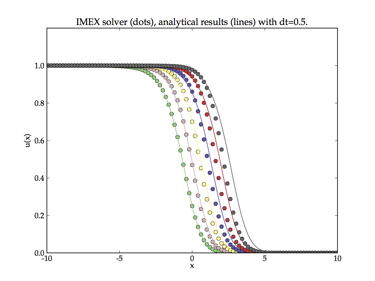
Solution of Fishers’ equation with an IMEX scheme.

Newton iteration

We have a semi-discretised system of the form \(u^{\prime}(t) = F(u(t))\) with the application of the \(\theta\)-method this gives,

\[w^{n+1} - w^{n} - (1-\theta) \tau F(w^n) - \theta\tau F(w^{n+1}) = 0\]

with unknown vector \(w^{n+1}\). This equation can be solved using Newton iteration.

\[\nu^{k+1} = \nu^{k} - (I - \theta\tau A^{n})^{-1} \left( \nu^{k} - u_{n} - (1-\theta) \tau F(w^n) - \theta\tau F(w^{n+1}) \right)\]

where \(k\) is the iteration index (\(k\geq0\)) and \(A^{n}\) is the Jacobian matrix of \(F(w^n)\). We use the symbol \(\nu^{k}\) for iteration variables such that they are distinguished from solution of the equation at a real time point \(u^n\). The iteration needs a starting value, it is perfectly value to choose \(\nu^0 = w^n\) or for a better estimate we can precompute one iteration \(\nu^0 = w^n + \tau F(w^{n})\). Here we have described the so-called modified Newton iteration because the Jacobian is not updated during the iteration, this is known to work well for stiff PDEs.

Applying the modified Newton iteration to Fisher’s equation yields the results shown in the Figure below. The results are much better than for IMEX scheme as the error (particularly for long time points) is much lower. However, the accumulation of global error can still be observed. This is a known feature of so called single step methods. In ODE terminology a single step method is one that uses only the most recent past data to evaluate the equation at the future time step. Note even if the equations are implicit (or semi-implicit as with the \(\theta\)-method) the future state is predicted only from one historic data point. In contrast a multistep method would used many previous data points to achieve highly accurate time integration.

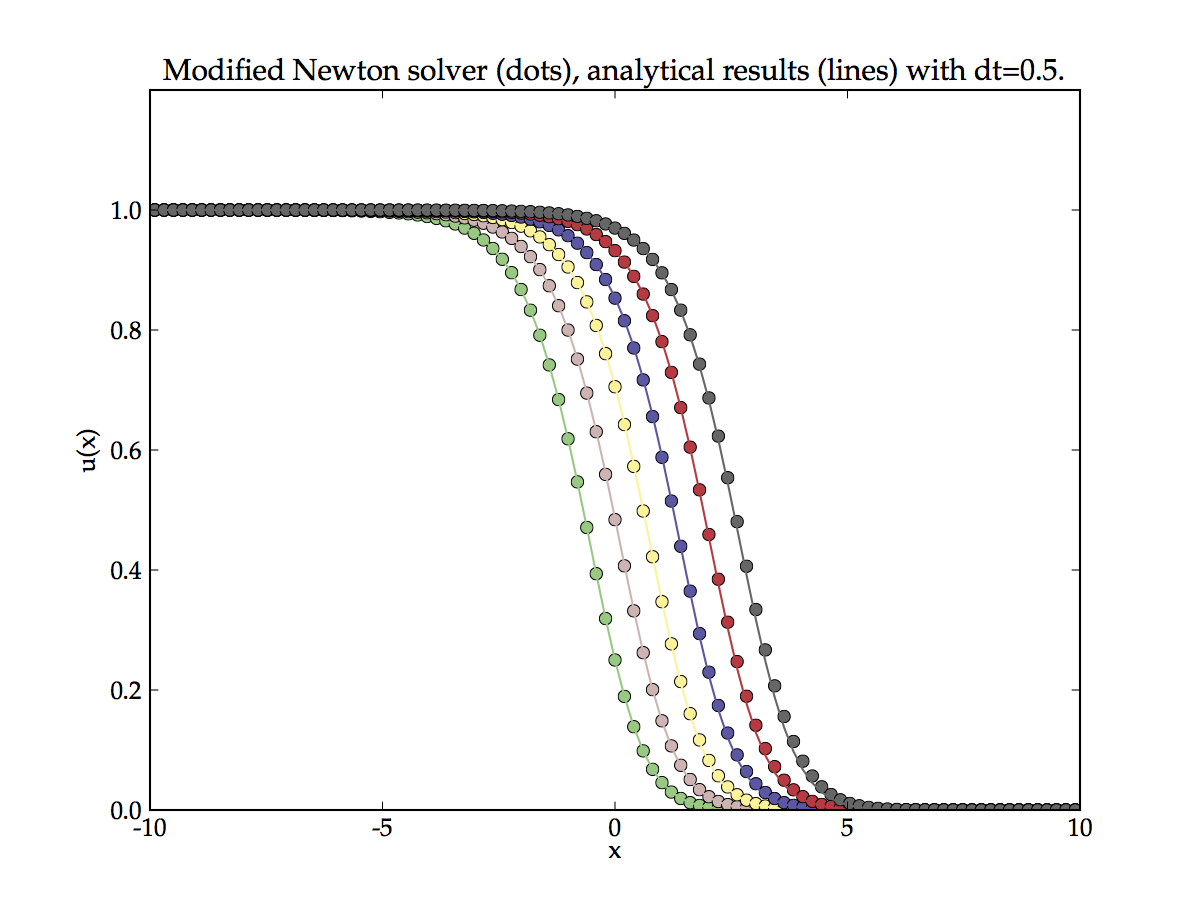
Solution of Fishers’ equation with a modified Newton iteration.

Method of lines

Note

For an excellent introduction to the Method of Lines see the article at scholarpedia.org

The method of lines is not really a method, it is a way of writing PDEs in such a way that they can be solved by black box ODE solvers. The time integration of ODEs is a mature topic. Robust and well tested solvers are readily available on the internet and integrated into many open-source projects for easy use. The method of lines is a way of letting PDE equation take advantage of the mature nature of ODE solvers.

We have a semi-discretised system of the form, \(u^{\prime}(t) = F(u(t))\) to use the method of lines we leave the PDE is the semi-discristed form such that is has a continuous time derivative on the l.h.s., i.e. \(u^{\prime}(t) = \frac{du(t)}{dt}\). In the semi-discretised form what we really have is no longer a PDE but a system of coupled ODEs. Moreover, a PDE equation is a differential equation which contains differential terms with respect to more that one variable. In this semi-discretised form we have replaced the spatial differential operator with a matrix so there is only one derivative. The equation has become a system of ODEs with number of equation proportional to the number of grid points in our discretisation.

Note

The discretised boundary conditions are expected to be included in \(F(u(t))\) such that the problem is well posed.

There are a wide variety of ODE solvers we are interested in the implicit type as we know many PDE problems are unstable in explicit form. The result in the Figure below have been calculated using an implicit multistep Adams-Moulton method (the algorithm used is the highly popular vode solver from netlib.org, although we used actually used a Python wrapper from scipy to perform the calculations shown). This can be thought of as a generalised of the \(\theta\)-method to include a multiple number of future time steps which are solved simultaneously with a Newtom iteration. Unlike single step method, multistep methods do not show a global error accumulation, so the time integration is a much better approximation to analytical solution. Fisher’s equation is not particularly stiff so this approach worked well. However for stiff equations a technique called Backward differentiation formulas (BDF) is used. The vode solver has the ability to dynamically adapt between stiff and non stiff mode (i.e. Adams-Moulton to BDF) which is one of the reasons for it’s popularity.

The method of lines is a powerful technique for solving semi-discretised PDE problems as much of the details of numerically solving the equation can be off loaded to mature and robust solvers. I do not yet have enough experience with the technique to point out short coming or failings. But it seems that provided the spatial discretisation is stable the details of the time integration can be almost ignored!

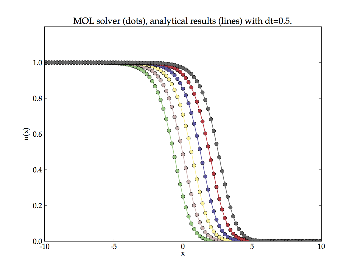
Solution of Fishers’ equation by the method of lines.