Boundary conditions for the advection-diffusion-reaction equation

The advection-diffusion-reaction equation is a particularly good equation to explore apply boundary conditions because it is a more general version of other equations. For example, the diffusion equation, the transport equation and the Poisson equation can all be recovered from this basic form. Moreover, by developing a general scheme for boundary conditions of the advection-reaction-diffusion equation we automatically get a system for imposing boundary conditions on all equations of a similar form.

Robin boundary conditions (known flux)

Robin specify a known total flux comprised of a diffusion and advection component. Note that in the diffusion equation limit (where \(a=0\)) these boundary conditions reduce to Neumann boundary conditions.

Within the finite volume method Robin boundary conditions are naturally resolved. This means that there is no need for interpolation or ghost point substitution (although these approaches remain possible) to include the boundary conditions because the flux at the boundary appears naturally in the semi-discretised equation. For example consider the semi-discretised equation evaluated at the boundary cell \(\Omega_1\),

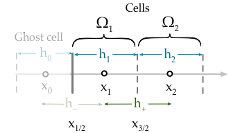
Finite volume boundary cell at the left hand side.

\[w_1^{\prime} = -\frac{\mathcal{F}_{3/2}}{h_1} + \frac{\mathcal{F}_{1/2}}{h_{1}} + \bar{s}_1\]

The Robin boundary condition specifies the flux at \(x_{1/2}\),

\[\mathcal{F}_{1/2} = g_{R}(x_{1/2})\]

Therefore the boundary condition can be incorporated without invoking any information regarding the ghost cell,

\[w_1^{\prime} = \frac{w_1}{h_1}\left( \frac{-a(x_{3/2})h_{2}}{2h_{+}} - \frac{d(x_{3/2})}{h_{+}} \right) + \frac{w_{2}}{h_1} \left( \frac{-a(x_{3/2}) h_1}{2h_{+}} + \frac{d(x_{3/2})}{h_{+}} \right) + \frac{g_{R}(x_L)}{h_1} + \bar{s}_1\]

Similarly applying the same procedure to the \(\Omega_J\) cell at the right hand side boundary,

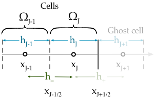
Finite volume boundary cell at the right hand side.

\[w_J^{\prime} = -\frac{\mathcal{F}_{J+1/2}}{h_J} + \frac{\mathcal{F}_{J-1/2}}{h_J} + \bar{s}_J\]

The Robin boundary condition at the right hand side is,

\[g_{R}(x_R) = \mathcal{F}_{J+1/2}\]

Therefore the naturally resolved boundary condition on the right hand side becomes,

\[w_J^{\prime} = \frac{w_{J-1}}{h_J}\left( \frac{a(x_{J-1/2})h_{J}}{2h_{-}} + \frac{d(x_{J-1/2})}{h_{-}} \right) + \frac{w_{J}}{h_J} \left( \frac{a(x_{J-1/2}) h_{J-1}}{2h_{-}} - \frac{d(x_{J-1/2})}{h_{-}} \right) - \frac{g_{R}(x_R)}{h_J} + \bar{s}_J\]

Dirichlet boundary conditions (known value)

Warning

This is only valid provided the initial conditions also satisfy the boundary conditions

Dirichlet (known value) boundary conditions are trivial to implement. All that is required is to fix the boundary term to be a constant value. If the initial conditions satisfy the boundary conditions (as they should) then all that is needed to to make sure that the time-derivative (the change with time) of the boundary points is always zero. For example, to impose Dirichlet boundary conditions

\[w_1^{n+1} = g_D(x_1) \quad w_{J}^{n+1} = g_D(x_J)\]

We simply need to specify,

\[F_1(w_1^{n}) = 0 \quad F_1(w_1^{n+1}) = 0\]

This can be achieved by multiplying the r.h.s. by the modified identity matrix where the first and last elements are zero,

\[w^{\prime} = \text{diag}(0,1,\cdots,1,0) \left( \theta F(w^{n+1}) + (1-\theta)F(w^{n}) \right)\]

If the boundary conditions are time dependent,

\[w_1^{n+1} = g_D(x_1, t_{n+1}) \quad w_{J}^{n+1} = g_D(x_J, t_{n+1})\]

The we should also add a matrix to the r.h.s. which is contains the changes to the boundary value between the time-steps,

\[w^{\prime} = \text{diag}(0,1,\cdots,1,0) \left( \theta F(w^{n+1}) + (1-\theta)F(w^{n}) \right) + \text{diag}(\Delta g_D(x_1), 0, \cdots, 0, \Delta g_D(x_J) )\]

where,

\[\begin{split}\Delta g_D(x_1) = g_D(x_1, t_{n+1}) - g_D(x_1, t_{n}) \\ \Delta g_D(x_J) = g_D(x_J, t_{n+1}) - g_D(x_J, t_{n})\end{split}\]

The following assumes time-invariant boundary conditions.

General matrix form with a transient term

The semi-discretised advection-diffusion-reaction equation can be written in the form below using the \(\theta\)-method,

\[w^{\prime} = \alpha\left( \theta F(w_j^{n+1}) + (1-\theta)F(w_j^{n}) \right) + \beta\]

where \(F(w)\) contains a matrix \(M\), a vector of the solution variable \(w\) and a vector of the reaction term \(r\),

\[F(w) = Mw + r\]

We have introduced a new matrix, \(\alpha\) and vector, \(\beta\). These are used to incorporate the boundary conditions, they have the form,

\[\begin{split}\alpha & = \text{diag}\left( \alpha_1, 1, \cdots, 1, \alpha_J \right) \\ \beta & = \left( \beta_1, 0, \cdots, 0, \beta_J \right)\end{split}\]

The modified coefficient matrix becomes,

\[\begin{split}M = \begin{align} \begin{pmatrix} b_1 & c_1 & & & 0 \\ r_a & r_b & r_c & & \\ && \ddots & \ddots & \ddots& \\ && & r_a & r_b & r_c \\ 0 && & & a_J & b_J \end{pmatrix} \end{align}\end{split}\]

Table showing coefficients which should be altered to apply either Robin or Dirichlet boundary conditions.

Symbol	Robin	Dirichlet
\(b_1\)	\(\frac{1}{h_1}\left( \frac{-a(x_{3/2})h_{2}}{2h_{+}} - \frac{d(x_{3/2})}{h_{+}} \right)\)	\(1\)
\(c_1\)	\(\frac{1}{h_1} \left( \frac{-a(x_{3/2}) h_1}{2h_{+}} + \frac{d(x_{3/2})}{h_{+}} \right)\)	\(0\)
\(a_J\)	\(\frac{1}{h_J}\left( \frac{a(x_{J-1/2})h_{J}}{2h_{-}} + \frac{d(x_{J-1/2})}{h_{-}} \right)\)	\(0\)
\(b_J\)	\(\frac{1}{h_J} \left( \frac{a(x_{J-1/2}) h_{J-1}}{2h_{-}} - \frac{d(x_{J-1/2})}{h_{-}} \right)\)	\(1\)
\(\alpha_1\)	\(1\)	\(0\)
\(\alpha_J\)	\(1\)	\(0\)
\(\beta_1\)	\(\frac{g_R(x_1)}{h_1}\)	\(0\)
\(\beta_J\)	\(-\frac{g_R(x_J)}{h_J}\)	\(0\)

General matrix form without a transient term

The boundary conditions scheme discussed above is only valid for initial value problems; problems where an initial vector of the solution variable \(w^0\) is specified along with boundary conditions. PDEs of the advection-diffusion-reaction form that do not contain a time derivative are an important class of equations they are called boundary value problems,

\[0 = \alpha\left( \theta F(w_j^{n+1}) + (1-\theta)F(w_j^{n}) \right) + \beta\]

Boundary value problems do not require initial conditions for the solution variable. For this type of equations we need to use a different general scheme to implement boundary condition values.

The element of the \(M\) matrix remain the same, however for Dirichlet boundary conditions the elements must be modified in for the \(\alpha\) and \(\beta\) terms,

Symbol	Robin	Dirichlet
\(\alpha_1\)	\(1\)	\(1\)
\(\alpha_J\)	\(1\)	\(1\)
\(\beta_1\)	\(\frac{g_R(x_1)}{h_1}\)	\(-r(x_1)- g_D(x_1)\)
\(\beta_J\)	\(-\frac{g_R(x_J)}{h_J}\)	\(-r(x_J)- g_D(x_J)\)